Lot Sizing Problem

We introduce the Lot Sizing Problem (LSP) as a General module use case

Introduction

The Lot Sizing Problem (LSP) is a production planning problem that has been traditionally addressed in the fields of management science and optimization. The decision maker wants to determine the amount of production that will satisfy the demand in each period of a given planning horizon while minimizing total cost (the sum of production cost, fixed cost, and inventory cost). Demand in a given period is satisfied by either production or inventory in that period. In the case of producing a product, there are fixed costs to run the production facility and variable costs that are proportional to the amount of production. In the case of inventory, there are maintenance costs.

Network of Lot Sizing Problem

Example

The following is a simple example of an LSP. Suppose you have five days of demand for a product and information about variable costs, fixed costs, and inventory costs as shown in the table below.

Info.	Day 1	Day 2	Day 3	Day 4	Day 5
Demand	3	2	1	2	1
Production cost	3	0	1	0	2
Fixed cost	0	12	7	4	5
Inventory cost	0	0	0	0	0

There are many possible solutions to the above problem, i.e., production plans that satisfy demand for five days.

Solution 1

Info.	Day 1	Day 2	Day 3	Day 4	Day 5
Production amount	3	2	1	2	1

Solution 1 above corresponds to a plan that produces only what is needed each day, in which case the total cost is calculated as follows.

$$\text{Cost} = (3 \times 3 + 0) + (2 \times 0 + 12) + (1 \times 1 + 7) + (2 \times 0 + 4) + (1 \times 2 + 5) = 40$$

Solution 2

Info.	Day 1	Day 2	Day 3	Day 4	Day 5
Production amount	5	0	1	2	1

On the other hand, for Solution 2 above, the plan is to produce the required amount on Day 1 and the next day, resulting in an inventory of 2. In this case, the total cost is calculated as follows

$$\text{Cost} = (5 \times 3 + 0) + 0 + (1 \times 1 + 7) + (2 \times 0 + 4) + (1 \times 2 + 5) = 34$$

Therefore, we can observe that Solution 2 is a better solution from a cost perspective than Solution 1.

Dynamic Programming

Characteristics of optimal solutions

The LSP can be modeled by dynamic planning methods, which exploit a unique property of LSPs: the structural characteristics of their optimal solutions. LSPs can be shown to have optimal solutions that satisfy the following properties.

Characteristics of LSP Optimal Solutions

1. Define $t_1,\cdots,t_r$ that satisfies $1 \leq t_1 < t_2 < \cdots < t_r \leq T$. The production amount in $t_j$ is $d_{t_j}+\cdots+d_{t_{j+1}-1}$ for $j$ where $1 \leq j \leq r$ . ($t_{r+1} = n+1$)

2. Only production occurs if the current inventory on hand is zero.

3. If production is made in period $t$, then the production amount is exactly equal to the total demand from $t$ to $t+k$ for any $k$ where $0 \leq k \leq T-t$.

This means that the periods in which production occurs are a subset of all periods, and that in each production period, you produce to satisfy exactly the demand from the current period to the period immediately preceding the next production period. Therefore, the inventory you have at the start of each production period is zero. A network representation of this would look like this: In Period 1, you produce to satisfy demand from Periods 1 through 3, and with zero inventory, you produce to satisfy demand from Period 4 through Period 5. The intervals $[1,3]$ and $[4,5]$ are called the regeneration intervals.

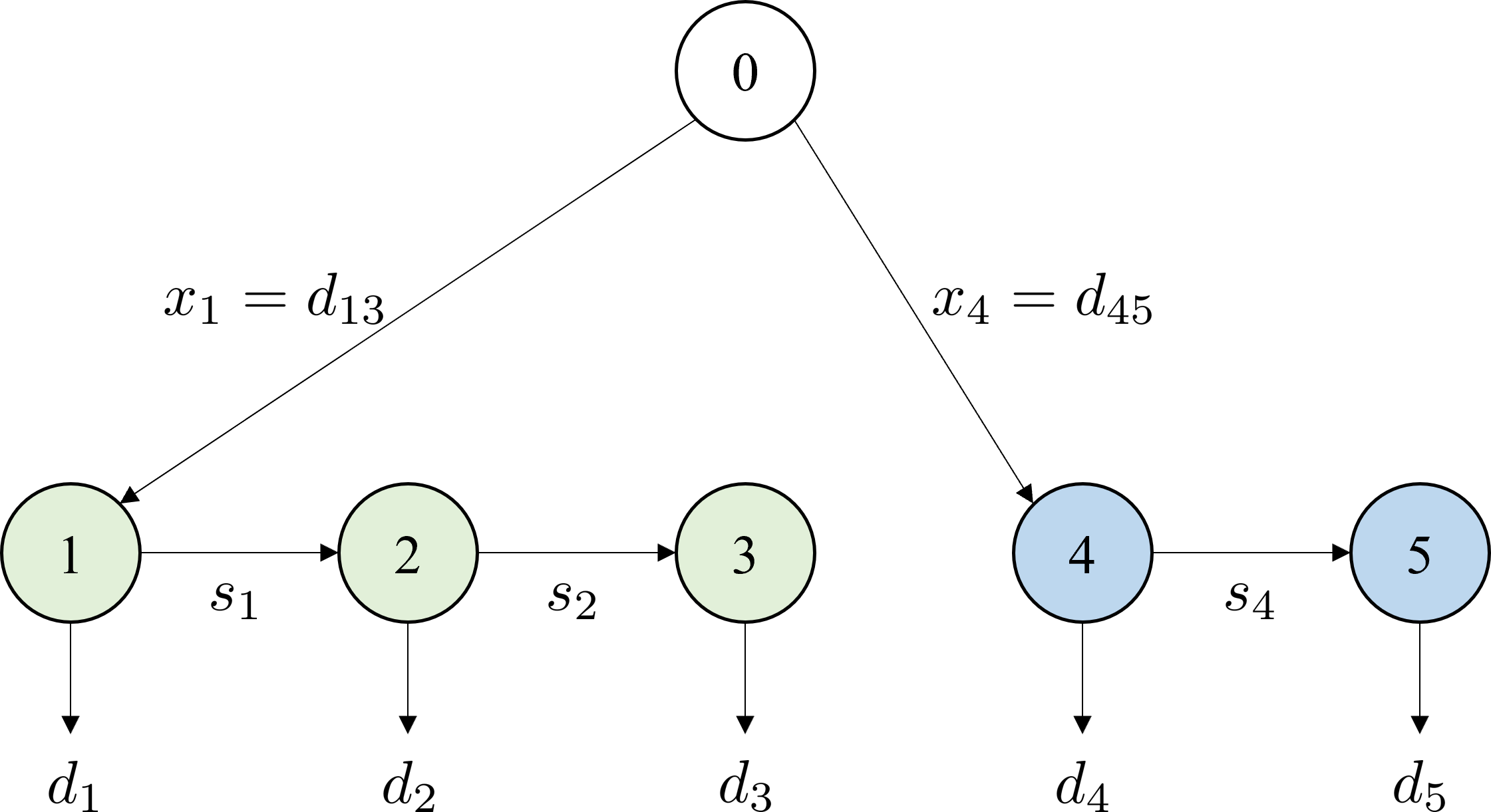
Structural characteristic of LSP optimal solutions

We use these characteristics to model the LSP as dynamic programming.

State

The state at stage $t$, which is not the final stage, is defined as the ordered pair$(k,t)$ for $k \leq t$. The state $(k,t)$ means that when solving the LSP from period 1 to $t$, $k$ is the period in which the last production occurred. That is, $[k,t]$is the last regeneration interval and the production in period $k$ is $d_k + \cdots + d_t$. Let $J(k,t)$ be the cost corresponding to each state, which represents the minimum cost of all the plans whose last regeneration interval is $[k,t]$.

Stage

The periods defined in the problem correspond to the stages. We additionally define a stage with a final state that indicates the termination, so the example above would have 6 (=5+1) stages.

Action and state transition

In state $(k,t)$ where $k \leq t < T$, there are two possible actions.

1. Include $t+1$ in the current regeneration interval $[k,t]$. In this case, a transition occurs from state $(k,t)$ to $(k,t+1)$. This means that we need to produce an additional demand $d_{t+1}$ in period $k$ that corresponds to $t+1$, incurring a transition cost of $p_k \cdot d_{t+1}$.

2. Start a new regeneration interval at $t+1$. In this case, a transition occurs from state $(k,t)$ to $(t+1, t+1)$. Since we are starting a new production in period $t+1$, we incur a transition cost of $q_{t+1}+p_{t+1} \cdot d_{t+1}$, which is the sum of the setup cost and the production cost.

The transition cost to the state of the last stage is defined as 0. A graphical representation of the above actions is shown below.

Possible actions in state (k,t)

The state transition network in the previous example is shown below.

State trasition network in LSP

A path from the initial state (Start node) to the final state (Final node) corresponds to a feasible solution to the problem, and the shortest path corresponds to the optimal solution to the problem. The path that represents the optimal solution is shown below.

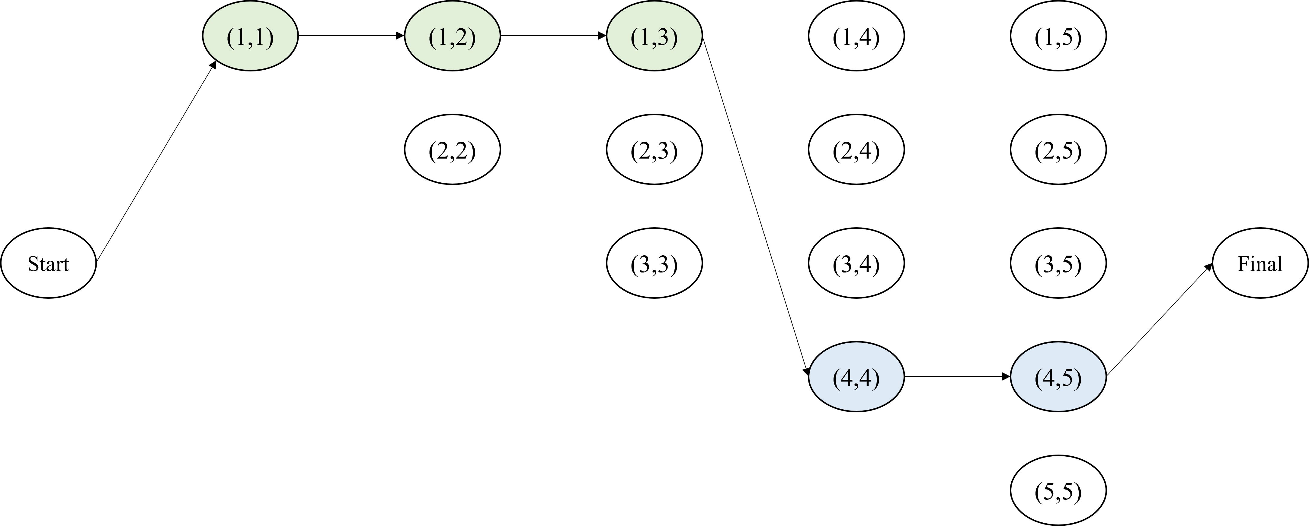
The optimal solution of the LSP and the corresponding shortest path on the network

DP Recursion

We denote the cost corresponding to each state by $J(k,t)$, which represents the minimum cost of the plans whose last production occurs in period $k$.

Let $G(t)$ be the minimum cost of the problem over period $t$, then we have

$$G(t) = \min_{k: \, k \leq t} \{J(k,t)\}.$$

The relationship between each state and the transition cost is defined as follows. (Define $G(0)=0$)

$$\begin{align*} &J(k,t+1) = J(k,t) + p_k d_{t+1} \qquad \text{for all } k,t \text{ with } k \leq t, \\ &J(t,t) = G(t-1)+q_t+p_td_t \qquad \text{for all } t. \end{align*}$$

How to solve the example problem

$G(1)=J(1,1)=0 + 3 \times 3=9$

$J(1,2)=J(1,1)+2 \times 3=15$

$J(2,2)=G(1) + 12 + 2 \times 0 = 21$, so $G(2) = \min \{ J(1,2), J(2,2)\} = 15$ holds.

$J(1,3)=J(1,2) + 3 = 18$

$J(2,3) = J(2,2) + 0 = 21$

$J(3,3)=G(2) + 7+1 \times 1 = 23$, so $G(3)=18$ holds.

We can find the optimal solution to this problem by computing $G(5)$ by forward recursion starting with $G(0)=0$ in the same way described above.

State Bounds

The bound information of the state can be used to reduce the search space to speed up the computation time to find the optimal solution, or to find an approximate solution.

Primal Bound

To find a primal bound on the state $(k,t)$, we need to find a feasible solution. There are several ways to find a feasible solution, the simplest of which is to group the remaining periods from $t+1$ to $T$ into a single regeneration interval. This feasible solution may not be optimal, in which case the primal bound is $J(k,t)+ q_{t+1} + p_{t+1}(d_{t+1}+\cdots + d_T)$.

Dual Bound

In order to find the dual bound at state $(k,t)$, we can solve a relaxed problem that relaxes some of the constraints in the problem. The simplest dual bound is to set all cost parameters to zero after time $t$. The dual bound obtained is $J(k,t)$ in this case. Several other relaxation techniques can be employed.

References

Production Planning by Mixed Integer Programming. Y. Pochet, L. Wolsey. Springer. 2006.